Measurement and Control, Regulation of Real processes in the world
What is the diameter of an atom or atomic nucleus? What is the size of an electron, what is the circuit of the Earth, how far is the Moon from the Earth and at what distance are the nearest stars from the Sun and many many more questions. Together with this questions should be followed by explanations as to how the previously mentioned values were measured – what was the principle of measurement, what units were used, what is the accuracy of the measurement methods, etc.
When we give objective values, such as the circumference of the Earth, we must specify the method used to measure it (Eratosthenes) and how it is possible to measure the circumference of the Earth without direct measurement. We must also specify the unit of measurement—the distance between two points on the Earth, a wooden or steel ruler with a fixed point, etc. Then we must specify the accuracy of the measurement depending on the scale and measurement method used. Only then do we give the measured value of the circumference of the Earth together with the tolerance range. Similarly, we determine the distance between the Earth and the Sun, or the Earth and the Moon, or the distance to the nearest stars using triangulation methods.
The same is valid for how to estimate the diameter of atom, atoms nuclei, distances in our galaxy, distances among galaxies, etc.
There are plenty measures in the world. All measurements are temporary. They have a limited validity. Roughly 99.8% of measurements are used in manufacturing, planning, and construction surveying. Their lifetime is limited to a few decades at most. The remaining 0.2% are measurements such as the circumference of the Earth, the distance between celestial bodies, the determination of sea levels (altimetry) and the world’s oceans using satellites, the size of atoms or molecules, and many other measurements. These measurements are valid for hundreds (or even thousands) of years. They are simply becoming more accurate over time. And then there are measurements of mutuality, of mutual relationships among objects and events—mutual relationships in terms of functionality or beauty. And it is precisely this type of “measurement”—if it can still be called measurement—that all measurements point to. To an understanding of mutual connections. There is not much of interest in atoms, but there is so much interest in molecules, let alone crystals and solids, that it is impossible to express (artistic and craft works, technical products, buildings, all of nature). In short, the purpose of all measurements is to increase knowledge, to realize the interrelationships among temporary objects and events, without any constants or fixed (unchanging) points. In fact, there are no fixed points in the universe at all. Even if we take the Greenwich Observatory as a fixed point, it is subject to geological changes, and all measurements are relative to a temporary (fictitious) fixed point.
The regulation of the system takes place in a chain – cause and effect. Only after a deviation occurs does the regulator activate the regulatory process to return the system to its original parameters (or nearly original).
The top is to control system before deviation will occur. To feel what will hapen on basis of past experience with given systems.
Before the actual measurement and control, it is necessary to mention the limits of mathematics.
The real world is always determined by a range of properties. A range of values – tolerances. Every form and event in the world is always changing. Even if we have a precisely manufactured rod or ball with the highest possible accuracy – yet the diameter of the ball is not constant, but varies within a certain range. Not only the range of manufacturing tolerance, but for example the thermal vibrations of molecules. These cannot be stopped.
In short, reality is always foggy. There is always a probability range – an unpredictable value in a given probability range. We do not and can never know the exact size of a ball or any other manufactured product or the realities of nature.
But Mathematics supposes stable (invariant) numbers. See base units. However, mathematics cannot be different by its very nature – the numbers 1, 2, 3, … , until infinity. The number 2 represents the sum of two equal (identical) values 1 . Mathematics, even if it calculates with real numbers, must round them to a limited number of decimal places. Such mathematics cannot be mindlessly applied in the real world, where no two entities are the same and moreover, they’re changing. Mathematical equations are valid for an ideal world, a world with ideal given changes. For a world removed from Reality, i.e. a dead world. And that’s what everyone who tries to evaluate the world with this idol look like. Mathematics is like language – only to direct us, to lead us to inexpressible and changing Reality. Nothing against equations, they are unmissable, but they must be subordinated to Reality and not vice versa.
The agreement of mathematical equations of idealized models with reality – see crank mechanism or pendulum. Likewise thermodynamics and many other examples. Many scientists were then literally fascinated by the mathematical possibilities which led them to explain or predict events in areas that could no longer be verified. See Archimedes, fascinated by the power of the lever to move the Earth. Which is theoretically and practically impossible.
Ideal models are valid, even 100% valid for given ideal conditions. The validity of the prediction is limited by the computational accuracy. So nothing against ideal models determining absolute temperature, the expansion time of the universe, or the position of the crank mechanism. One can take into consideration a real crank mechanism – determine (scan) the dimensions of the connecting rod, piston and other parts, determine the structures of the materials used, the locations of the greatest forces and thus the locations of breakage or wear. At the point of sliding movement – the greater the tightness the greater the accuracy but also the greater the wear and the greater the freedom in sliding the less the accuracy but also the worse the wear. Precisely because mechanisms, like all processes in the universe, are subject to wear. Even if we determine the point of highest wear, we cannot determine the exact location of the wear and its progression. It will always have a probabilistic course. In other words, a random, unpredictable element will enter into the idealized real mechanism, or predictable, but within a certain range. This range will be many orders of magnitude away from the original accuracy of the calculation (scan of dimensions, positions of interacting parts, etc.). Thus, the original high accuracy of the idealized real mechanism will be fatally broken. The accuracy of the prediction will be completely off in this case as well.
For an idealized crank mechanism from an ideal steel, we can predict for millions of years or billions of years with sufficient accuracy. It is not possible to predict the position of a real crank mechanism for x-turn, let alone for x-days or years. We don’t know what will happen. The same is true for all mechanisms. No two steels are exactly the same even if they are in the same category under the same code. The same code provides validity of mechanical properties to 98% or 99.98%, but these steels are very expensive. The greater the simplification from reality, the greater the illustration and clarity, but the shorter the validity of the prediction over time. Not to mention – weather forecast for ½ year or 10 mil. years. We know „exactly“ the weather on Mars, we „exactly“ know processes in the beginning of our universe, but we are unable to predict weather report more then several days. Not to mention so-called three body problem in mechanics.
E.g. a projectile movement in various unpredictable chaotic environments – see the foggy background of our world, different atmospheric conditions through the path of the projectile – to predict the future path or estimate the past one at a given accuracy, it´s a big problem. However, in ideal conditions, where there is no atmosphere, it is quite easy. That’s what gunners would like, perhaps on the Moon.
Conclusion: The projectile must have a control system to correct its trajectory. Similarly, theories, no matter how “perfect”, have to be verified, otherwise they are not very meaningful.
The accuracy has its own limits – fluctuations of omnipresent chaotic environment.
Measurement and control is necessary in the real world. Every process in the reality must be controlled. And measurement, including follow-up control, is based on observation, on the use of measurement – the comparison of base units with measured values. Permanent verifiability. Process control – the basis for everything – see Adaptability, Complexity, Proportion, Reciprocity. There must be limits in the range of the control. The range of control means the possible states, the deviations, etc. The range is given by detailed calculations. Without these calculations no process control is possible. It is absurd, on the basis of idealized models, to predict the operation of a crank mechanism for hundreds of days or years, or to predict events in astrophysics for billions of years without observation. Nothing against idealization and initial calculation, one has to start somewhere, but one has to know this and go further according to experience with Reality, verifiable Reality.
Measurement, probability and statistics
What is the correct value? The correct value is the measured value. Whether it’s the most frequent value, or the average of the values, or the median, it doesn’t matter. But the correct value is always the measured value. And it always varies slightly. We will want to know, yes we have measured something, but what is the real, the right value. There is no real, right or correct value at all. The correct value is the measured value, whether the value with the most frequent occurrence or the averaged value, it does not matter, the correct value corresponds to the measured value. And the measured value is just like the “correct” value, “both” are only temporary and doesn’t actually exist, always changing slightly over the lifetime of the measured object or event. There is no right or correct fixed value from outside. The reason for repeated changes in the measured values are omnipresent fluctuations. From the set of slightly different values the most frequent value is chosen as the “correct” value. This is how all values (diameters, distances, intensities, frequencies, etc.) change, including fundamental physical constants such as the speed of light c, Planck’s constant h, or the gravitational constant G.
Where is the correct (right) value N? We are unable to measure directly correct (given) value N of something – diameters of balls or anything else. We are only able to measure a certain amount of values that, in effect, when plotted, resemble Gauss’s distribution curve of random errors. In other words, we consider the peak of this curve to be the right value N. Or the most frequent value becomes the right value N. See below
Measured values oscillate at interval N ± d over the “right” value N, which is irrational (see rational numbers oscillate around irrational ones to infinity) and, crucially, the indescribable right value N keep changing – it’s “alive”.
The prove – the Gaussian distribution curve also oscillates, slightly, through the time, when we take several sets of measurements of the value N – e.g. a diameter of a ball. We could say “Probability of probabilities”. We don’t measure all values at the same time, but we measure sequentially over time. Each value has its own time when it was measured. The measured values change – they oscillate with the frequency of their appearance according to the Gaussian curve of the frequency distribution of the measured values. Each value differs both in value and in the time at which it was measured. It cannot all happen at once for a matter where there is a difference between time and distance. That would not be matter then, but radiation, where there is no difference between time and distance.
How to determine the pitch (frequency) of a tone and its duration (from the moment it begins to the moment it ends) ? To determine the value, we need at least a few completed cycles. See below
![]()
It is
Microlevel – fast changes in spite of macrolevel – slow changes. Both changes are indescribable.
Upper mentioned images are taken out from following illustration of natural processes
Let´s go to the emission of light. E.g. the wavelenght N of emitted light from hydrogen atom. Specifically, the line spectra, so characteristic of each element from hydrogen, helium, through sodium, etc. The line spectrum needs to be taken realistically and not strictly mathematically. There is no ideal line without thickness in the world, just as there is no ideal point or ideal circle. Reality, then, is always a bit of a blur. It follows that our measurements are inaccurate. Nor is there an absolutely sharp scratch of the measuring instrument. Thus, even the so-called sharp line spectrum of emitted light has a very small yet fuzzy nature. It is best expressed again by the Gaussian distribution curve.
We will never measure two identical values at the wavelength level of light – see orange lines in an image below. Light is part of an ocean of quantum field full of random quantum fluctuations. Never repeatable. The idea for theory of dissipation or irreversibility.
We take the distance between two peaks h of the two curves for the value of the “correct” wavelength. It should be added that there is no exact value of the wavelength of light emitted, for this nature – a kind of blurism is inherent in the nature of real nature in and around us. So it would be better to no longer call this attribute, in the form of a mathematical notation and graph, the distribution curve of measurement errors. However, this is a natural characteristic of real nature. We also don’t call the error the movement of molecules or we don’t call the error the range of the oscillating movement of the spring. Would we then call the movement of an elephant or a human in a restricted place the error? However, it is meant to sit in the middle and not walk at different distances from chair to room? Or shall we call pregnancy a disease?
It should be remembered that the calculation of Planck’s constant was done in the above mentioned way. The same way as the calculation of the gravitational constant or the speed of light. There have always been a range of accuracy in the calculated values. Now the calculated values were taken to be invariant. But in reality they are not constant in a changing world. The point is that simplification through the fixation of fundamental constants can bring later complications.
Certainly the logic of fixing the base constants is clear. The constant is fixed to a certain value and the other values change with a much larger tolerance range. This is exactly what makes this method misleading. Even a unit is subject to change and these changes (tolerance range) cannot always be included in derived or interacting variables.
When we measure the dimension of an object, we measure it with a certain final accuracy. The final accuracy is determined by the sum of the accuracy of the measuring instrument and the accuracy, stability of the object to be measured. See below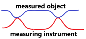
We measure the distance under probability distribution of values by ruler under probability distribution of its accuracy. There is no fixed distance in nature at all. Each measurement of e.g. the distance will be slightly different just because of the elastic deformations of the measuring device and the measured object. This is best seen by replacing the gauges with a spring with a certain very high stiffness. The resulting measurement accuracy (in the case of length), the of the measured values, consists of four parts, two parts are given by the measuring instrument and the other two parts are given by measured object. Even if we measure from one side, the other side must be supported somewhere, otherwise we would accelerate the object instead of measuring it.
If we measure Johansson’s gauges with a caliper, the accuracy of the gauges comes out low. If we measure the same gauges intereferometrically, we get excellent accuracy. If we use more precisely method (ionic projection) then we obtain stochastic course of measured value. In fact, “accuracy” disappears. Again a problem – we have to choose the most frequent value or the most average value – see evaluation of measurements.
In the case of ultra-high precision, the influence of energy is quite significant. The smaller the wavelength of the radiation used, the greater the accuracy of the measurement. However, the greater the energy of the radiation, the greater the influence on the measuring accuracy – see the use of very short wavelengths with high energy. See below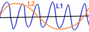
The wavelenght L1<L2 wavelenght. Then the wavelenght L1 has the greater resolving power relative to smaller wvalenght L2. But in the case of L1 there is greater influence of measured object. There is a rule – if we measure then we deform.
Anyway – we measure chaotic environments bound into e.g. solids by chaotic equipments bound into rulers. There is no ideal ruler in the world at all.
See also surface roughness of technical materials. The bigger polished steel ball the more accurate diameter. In short, the roughness of the polishing remains the same, but relative to the larger diameter will be an increase in relative accuracy.
Measurement – to find out the right value e.g. the distance between two real points. If we use the maximal accuracy we measure variances (oscillations) of these fluctuations (blue) around an “imaginary” value—the so-called right value (orange). See below
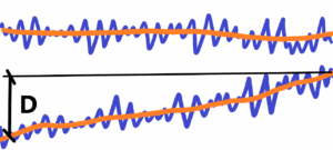
Such precision can be considered unnecessary, like empty magnification in telescopes or microscopes. To only know the course of the “right” value (orange), if there is a change or not. The decisive criterion is the difference D measured between the same points over a time interval. If D> max. dispersion (blue), then there is a change in macrostate like the distance between two points.
All Nature appears to us always in probability distribution (appearances) of measured parameters. It’s as if everything is hidden in the fog of randomness. But that randomness has quite well-defined areas – see probability appearances all distinguishable shapes, forms or events (processes). The well-known we can also get the Gaussian normal distribution curve in another way. See below
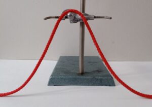
See the upper rope on the support. As can be seen, here probability has no meaning, nor randomness, but only necessity. The shape of the rope is very close to a Gaussian curve. However, this shape can change just as the shape of the Gaussian curve changes. Depending on the stiffness of the rope, the elevation of the support, etc. See below – different courses with different supported ropes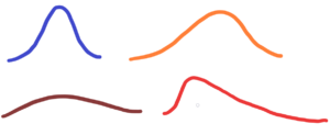
The blue rope has the same stiffness along its entire length. The orange rope has a higher stiffness on its left side. The brown rope has a greater stiffness than the blue rope along its entire length. Whereas the red rope has a high stiffness on its right side and a low stiffness on its left side. Thus, by using different ropes with different stiffnesses, we can get all possible combinations of probability frequency distributions – density functions.
Resolution versus regulation. It’s impossible to regulate processes that we can’t distinguish. For regulation, we need a distinguishable impulse. The more precise the scale, the more precise the regulation. However, there is some regulatory limit, or limit of distinguishability, not only for optical instruments in terms of diffraction, or the thermal movement of molecules, but above all the fundamental law of quantum mechanics – the Heisenberg uncertainty principle.
What can I say? When we want fine regulation we have to make fine differentiation. But that’s the trouble. Fine resolution requires short wavelengths for the observation process. See microscope resolution – the shorter the wavelength of the light used the greater the resolution. In other words, we see more details under blue light than under red light. If we use ultraviolet light or an electron microscope, we can very finely resolve even the smallest details that were previously indistinguishable. But there’s a problem. And that problem is the energy of the radiation used. At the beginning, we wanted fine control, so we want finesse, too fine. But to get fine resolution means using high-energy radiation. And high-energy radiation will greatly influence the object or the event we observe. So what we observe will have nothing to do with the initial event. Roughly speaking, if we want to work finer details in practice, we will have to use a stronger hammer. And that’s incompatible with finesse.
So, there are control limits from which we can get a certain optimum for a given control procedure together with the surrounding conditions.
Every shape, form, object has its own tolerance range. Even if systematic errors are excluded, random errors remain. Every most the most precisely manufactured object, component has a tolerance range, even if it is the slightest. But these errors are no longer errors in the classicsense, but the natural behaviour of all material objects – see thermal fluctuations of molecules. And they cannot be excluded by definition.
The longer the part the less accurate? Or the shorter the part the less precision? Due to the thermal expansion of e.g. steel, a 1 km long component will expand by approx. 1.2 m when heated at 100°C. A 1 mm long steel component will expand by approx. 1 micrometer. What about a component of a size comparable to the size of the molecules? That, when heated to 100°C… Anyway, think about constant temperature – every object, every measured object has its own temperature, its own trembling of its inner particles. There is no way to exclude them.
We see there are macrocomponents and microcomponents. For microcomponents, the tolerance range can be equal to, if not greater than, the size of the component at a certain temperature.
Notice: If the measurement results are loaded only by random errors, then the accuracy can be improved by increasing the number of repeated measurements. However, sometimes it is not advisable to take too many measurements because such measurements take so long that conditions may change and affect the result to an extent that cannot be estimated. As a general rule, a number of measurements not exceeding 10 should be made to show the accuracy with which the result of several repeated measurements is determined.
How to determine the middle value of random variables. Not just dimensions, but also surface roughness, for example. Let’s take the example of clocks that are either fast or slow, or alternately fast and slow – see temperature fluctuations together with material wear, including friction in bearings. Clocks have a certain tolerance of accuracy relative to one day. See accuracy +-1 sec/day or +-1 minute/day. If we leave the clocks alone, without occasional correction, what will happen?
There are three possibilities:
1) constant running fast, then the difference between solar noon and 12 o’clock on the clock will become greater and greater
2) constant delay, difference as above in point 1
3) running fast and slow, but here no one can guarantee that the average value for a certain period of time will be 12 o’clock on the clock versus solar noon (adjusted for the season).
To what extent should the stability of the operation be evaluated, will the mean value be maintained, or will it also change? It will certainly change if we leave the clock without correction. And for correction there have to be external clocks, or Solar noon or mutual positions of stars, etc.
The world, the universe It is about control, regulation, continuous adjustment, and balancing optimal values. It seems to be very easy solution for to transfer the body m from its initial position into its final position. See below
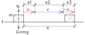
It is very easy to calculate this example mathematically. Firstly to acellerate the body m to suitable velocity and finally to decellerate body at along the desired path s. But how to do that practically? Without regulation, it’s impossible. There is no chance for randomness, for chaotic behaviour – only to regulate, to control the chaotic circumstances to the desired state. Select the area with the body and then proceed. Proceed either through an external energy or through one’s own energy—the mechanism of the human body—human being. In the end there have to be a will, the effort of the human being. Not only to think I will move with my hand, but the real effort by signals from neurons.
Thus, moving an object placed on a surface by a certain distance involves a great many processes. Where to obtain the energy for the movement, and how and by what means to regulate it. Energy always arises from the difference between two different potentials (hotter vs. colder, differences in water levels, pressures, forces and stresses, chemical potentials, etc.). Thus, it is not only a matter of seeking a sufficient amount of energy, but primarily of regulating it—controlling it.
Try to solve following question – see bellow
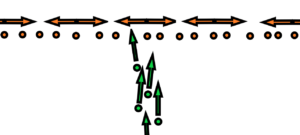
There are N balls. Every of them is oscillating around its zero position with max velocity u without the contact with the next ball. These balls are kept together in the frame with the same distance L. Against these balls are fired projectiles with velocity v. The weight of each ball is M, the weight of each projectile is also M. Collisions can occur when projectiles pass by oscillating balls. Or the diameters d of the balls as well as the projectiles are very, very small relative to the distance L.
The result of the experiment will be a distribution of projectiles on the screen surrounding the whole system in a circle.
The question is – will the distribution of projectiles on the screen change depending on the speed of oscillation of the balls? Respectively, will there be a significant difference in the distribution of projectiles on the screen depending on whether the balls are at rest or in motion?
Very interesting consideration about expanding air with inner grouped structures. There is a free speed c always equal to thermal speed of air´s particles. And there is bond particles into different structures. The speed of such particles is always less then c.
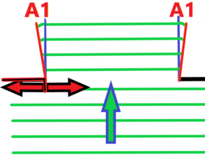
Very short remark about difraction. It is on diffraction that the resolving power depends. Diffraction – the bending of light passing through an hole, the bending of light on an edge or between edges differently distant from each other – See below
three black holes different in diameter, light waves in green, angles of diffraction A1 < A2 < A3
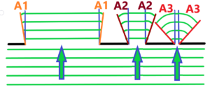
What do we see from the top picture? The smaller the diameter of the hole, the greater the bending of the light. The greater the edge distance, the less bending of the light, the less diffraction. Now imagine a hole with a variable edge distance. See below – with red marked arrows
We already know what will happen if we reduce the distance between the holes – the bending of light will increase. And if we extend the distance, we know that as well, the bending of light will decrease. Of course, all of the above cases apply to light waves that are nearly parallel or have an ultra-high radius. It is clear that the wave nature of light will be influenced by the interaction between the edge and light waves, or any electromagnetic waves – see radio waves.
And what if there’s only one edge? Does the bending of the light stop? Hardly, but we know that the resulting light wavefield is made of individual spherical wavefields. And if there are many spherical wavefields side by side, the resulting wavefield will be nearly parallel.
It is clear that the situation is somewhat reminiscent of the material bodies, the larger the dimension of the body in relation to the basic particles-waves of which the body is made up, the smaller are the expressions of the wave-particle nature.
Go on – we have an optical system made up of a lens with a certain aperture diameter. The lens has a focal length f where all the rays are focused. See below
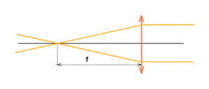
But beware of singularity. All radiation with a certain density will join together at one point, where an infinite density of radiation will then be. Yes, this is a nonsense. There is no ideal point, no ideal lens, no ideal conditions. Yes, it is possible to fire a paper or a cotton by lens with focused light, but without singularity.
In the upper mentioned system we will metion especially about the resolution and depth of field, or sharpness. The resolving power, like the depth of field, is related to a certain minimum size, a certain minimum quantum. Either the size of a single sensor element or the wavelength of the radiation together with a given aperture number. See below the image with the minimal size of the sensor element. E.g. one pixel marked red.
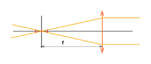
We can see that the size of one scan pixel influences the position tolerance of the whole sensor like CCD, etc. Depth of field as well as sharpness is determined by the sensor size, aperture diameter, focal length and wavelength of the light used. See below the tolerance
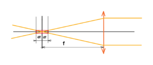
See below the tolerance of the complete sensor placing is given by twice the df. The smaller the pixel the smaller the depth of field at a given aperture. Then if we want to keep the depth of field for smaller pixel we have to increase the aperture number, i.e. decrease the aperture diameter. Limit state – When the aperture diameter is equal to the pixel size, then we can place the film or CCD sensor anywhere.
to be continued …
| Download | Download | Download | Download |
| Resolving_power_regulation | Measurement | ||