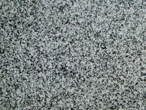
It would be better to write in the order of randomness, probability and necessity. For at the beginning is randomness of pure chaotic behaviour then the probability of the states or events and at the end necessity od states, forms or events. Such is already a feature of our world, a feature of the first primordial forms in the beginning of our universe – a matter field, or a quantum field full of chaotic random fluctuations – pure randomness of ever different “forms and “events”. Each situation is different, unrepeatable to each other and yet as a whole these situations look the same boring – see the grain on an untuned TV. See below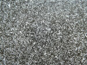
Pure randomness in a purely chaotic environment like the matter (quantum) field. Such a field permeates our entire universe. And all objects and events around us and within us are the result of renewed field excitations. There is no problem to obtain pure randomnes. But there are a lot of objects, forms and events with some certain appearances. See solids, liquids, gases. All the previously mentioned states of matter behave chaotically within themselves due to thermal fluctuations. I will ignore the matter (quantum) field fluctuations for now. If we were to look very closely at the previously mentioned states of matter, we would again see chaotic behaviour. Only for solids the chaos would be bound around an equilibrium position, for liquids the equilibrium position would be somewhat more extended, and for gases the chaos would be complete (unless the gas flows more or less in the same direction). And that brings us to coherence. Coherence in flow of liquids or gases through the pipes or there are many coherent sources like classical LC oscillator until maser or laser. Bulbs or discharge lamps or LEDs are not a coherent light source.
But it is absolutely clear that without bound thermal fluctuations (for example around the equilibrium position in solids) there would be no coherence, no coherent sources such as LC oscillators, quantum generators (masers and lasers) and for example in mechanics pendulums.
The world (univese) is full of chaotic behaviour. All solids, liquids and gases. Alongside pure chaos, there are “islands” of chaos flowing in the prevailing direction in the world. The flow of the chaos in one prevailing direction. E.g. the electric current (the flow of chaotic electrons through the wire, the flow of liquids or gases, the sounds waves, the movement of one body in a given direction and the “flow” of ELMG waves). But these “islands” are connected with in an all-around chaotic environment.
Mathematical models of natural processes for a long time have one very big disadvantage—they do not consider the influences of next events, i.e., events outside the horizon). We remember these physical laws were derived for every separated situation from isolated conditions without inner and outer “random” influences. In the same way were derived so-called probability laws – isolated conditions from “random” influences. We know what hard work is to find out the real RANDOM process in the world. E.g. also Brown motion is subordinated for a long time to its holder (flower, can, outer turbulences, etc.). Chaotic behaviour like turbulent flow in pipeline is subordinated to pipeline route. There is the necessity there.
It is clear from the above that all appearances of all differentiable solids, liquids, shapes, waves, structures, events or processes have probabilistic distribution.
So we’ll go to classical probability. I just want to point out that if the ball were not centered as much as possible with respect to the edge of Galton’s plate, probability phenomena would not occur. In short, when you throw the ball sideways, you get a certain, actually a necessity instead of a probability distribution of random variables.
Let’s go straight to the Galton board – very carefully prepared conditions – very unusual in nature.
We have an example:
16 balls passing through Galton board – the direction to the right is marked I, to the left 0
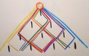
See an image below – there is the Galton board with 4 rows.
1 2 3 4 5
There are 5 boxes with 16 possible travel paths (differently coloured). Think an ideal state of probability – 6 different paths lead (are directed) to box 3, 4 different paths are directed to box box 5, 4 different paths to box 2, 1 same path (IIII) is directed to box 6 and 1 same path (0000) is directed to box 1. The final results of possible paths are given in following table – see below
| 0000 | 0I00 | I000 | II00 |
| 000I | 0I0I | I00I | II0I |
| 00I0 | 0II0 | I0I0 | III0 |
| 00II | 0III | I0II | IIII |
As we see the occurency (frequency) of possible travel paths are the same. Blue marked. There are 16 independent travel paths through Galton board. See an image below
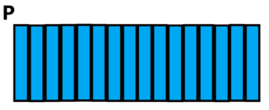
All paths has the same value. See upper image with 16 same identical rectangles – probability distribution. The probability value P is the same for all 16 events. Pure line of “density function” without any curvature. There is no preferred path of balls passing through Galton’s board.
When betting on the lottery, hardly any person will choose the number combination 11111111 or 44444444. The vast majority of people will choose the numbers 27543764 or 17329546 or something else. Because the probability of 8 identical numbers in a lottery is, in their opinion, vanishingly small. That’s true, but it’s also true that their chosen numbers has the same probability as 8 identical numbers. In other words, each different number arrangement has the same (very low) probability of winning.
But have a look at the upper table closely. We see that the probability of a number series with different numbers is more and more greater than the probability of a number series with 1 repeating number (in this case I or 0). In other words we see different occupations of the lower boxes by passed balls. That´s reality. See the next table below (differently coloured) – green colour for the results with one difference, red colour for results with no difference, deep gray colour for results with two difference.
| 0000 | 0I00 | I000 | II00 |
| 000I | 0I0I | I00I | I0II |
| 00I0 | 0II0 | I0I0 | III0 |
| 00II | 0III | I0II | IIII |
The probability of a result with alternating numbers is greater than the probability of a result with one repeating number. The more repetitions the greater the probability. See below the distribution based on upper table
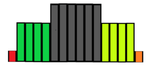
The distribution is quite different from constant distribution. What is the reason for this difference? However, the probability of each pass is always the same, constant. This is true, but the balls are grouped into one box regardless of the differences in their passage through Galton’s board. Grouping of different paths, different events into one place (box) is the reason why we get non-uniform curve distribution curve of frequency of occurrence (density function).
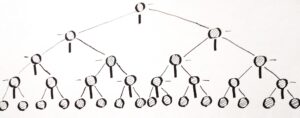
See below the Galton board with 10 rows and with 11 lower boxes
The distribution of passed balls through such board is illustrated on the upper second image. What is the conclusion? Without collection boxes, without limited spaces into which different events are collected, there would be no observable differences. See differentiability (distinguishability) – the resolving power of people or devices.
Probability to be of use requires distinguishability. Distinguishability of possible events.
Difficult to solve the probability of events on a continuum, where there are no clearly distinguishable possibilities. See the probability of one side falling on a dodecahedron. The probability is 1 to 20. For N-polyhedron, the probability is 1 to N. But at the ball? How to define the side? However, the side will be one point or one small area. Never fall the same deformed side for a real (deformable) ball or one point for an ideal ball. In this case, probability is not calculable. Do not mention the continuum distribution where a certain interval must be artificially created where the event occurs. So the first condition is the presence of stabilized and distinguishable sides, shapes, events or intervals – it doesn’t matter what we call them. This is what we silently suppose, and this is the basis of the probability calculus. Thus, before there was a probability there must have been distinguishable and stabilized structures – so called initial conditions. Probability is therefore a product of initial conditions. Probability cannot explain initial conditions by itself, only to use them properly. The initial conditions more closely correspond to the case of the falling ball. Every “side” of dropped ball is different to each other. There are no clear boundaries (sides). The reason is the irreversibility of processes. If we put a real manufactured ball through measurements of falls – one side will never be repeated. Every time we feel that one side has repeated, we will look closer and see a difference at the molecular level due to thermal motion. The same is true at the quantum level. No two events are identical. Then if we want two so-called identical events, or sides, we have to work the ball into an N-polyhedron. To cancel the expressions of molecular motion to such a level that there is a clear distinguishability – definability of the relevant sides. We must cancel the expressions of irreversibility.
Irreversibility is the basic principle of the Universe. See quantum field with “zero” vacuum fluctuations – completely random and indescribable changes inside that. Still unpredictably “bubbling”. Pure chaos. It’s impossible to get back a reverse motion exactly in such circumstances. Everything is always different and new. Although at first glance it might look the same. Here we have the very important question of how stabilized (regular and predictable) and differentiateable structures can exist in the middle of such a random and indescribable quantum field – see waves, particles, crystals, organisms, etc. These stabilized shapes, structures and processes in the world are always in change, in a slight change but always changing – no two snowflakes are exactly the same throughout the history of the Earth. Like all atmospheric conditions, clouds, every individual of the same species is different from other individuals in the same species. Sure – it looks the same in a first view, but only in a first view, in reality all of nature is still developing – see the Cambrian organisms compared to the Devonian organisms, and both compared to the present organisms.
Each snowflake is different from the others. No two snowflakes are the alike. But all snowflakes have a common characteristic, a common expression of their existence – a hexagonal configuration. Consider snowflakes or every roll of the dice. Every roll of the dice is unique. Surely the dice will land on 1 of the 6 sides. But if we observe and record the process of each dice roll, no matter which side it ends up landing on, we will find that the process of each roll is different – movement versus rotation. Even if we make trillions upon trillions of dice rolls, each roll will be a unique unrepeteable original. This reminds us of the origin – the indescribable and unrepeatable, purely random processes of vacuum fluctuations in the quantum field.
See the motion of an electron around an atomic nucleus. A closer look at the trajectory of the electron would show chaotic irregularities caused by quantum fluctuations in the electric field. The average deviation from the global trajectory is zero, but the root mean square deviation leads to a small shift in the energy level. This shift has indeed been measured as part of the Lamb-Retherford shift.
Each snowflake is different from all others, but each electron is different in its motion from all other moving electrons in the entire universe. And what electrons there must be in the universe! And this leads me to the final conclusion that each vacuum fluctuation is different from all vacuum fluctuations throughout the history of the universe
And again the question, in such a chaotic quantum field environment, where did the cubes (crystals) come from with their sides to fall on? What is repeatability and non-repeatability? See roll of the dice. How many rolls, so many unrepeatable and indescribable processes. But in the end, every dice always lands on 1 of the 6 sides. It’s hard to stay on the edge – a very unstable position.
So is the dice roll repeatable or unrepeatable? In terms of microstates, every roll of the dice is non-repeatable. In terms of the macro states, every roll of the dice is repeatable, predictable within the given possibilities – in this case 6 sides of the dice. For every roll of the dice we need a dice, so we need shapes, distances – in short, space. And we also need time – see each roll of the dice indicates a time duration (repeated oscillation changes). Briefly – Probability needs time and space and distinguishable shapes (subjects) inside. And again the question – where did time and space and distinguishable “regular” shapes or structures come from?
A temporary conclusion? It is not possible to return to the past, but it is possible to change the future, just on the basis of the past. In other words the arrow of time is a given and the impossibility of a time machine also.
Irreversibility, quantum field and the arrow of time
The chaos as we know is unstable. Chaotic behaviour is kept together by boundary conditions. Without boundary conditions there is no chaotic behaviour – no chaotic environment. See thermal motion, fluctuations of molecules – Brown fluctuations. In such „thermal“ environment there is complete chaos, unpredictable, incalculable, purely random. No two events are exactly the same – exactly the same in terms of position or momentum of particles. After all, each particle is different from other particles. The difference among them is inexpressible – see irrational numbers. Thus we have described the macroworld, the macrostate of thermal fluctuations. We suppose every fluctuation is non-repeteable original. Through all history of the universe.
Just like every snowflake is a non-repeatable original even though they have the same basic hexagonal structure. And what snowflakes have been created throughout the history of planet Earth. There is no problem to differ in details. We know from mathematics – there are infinity numbers between two any closer points.
Let´s go to the microworld, better to write to the microstate. The universe is filled with an elementary quantum field. In the quantum field there are violent changes of „shapes“ etc. These changes are called vacuum fluctuations. See an image below.
We suppose every fluctuation inside quantum field is non-repeteable original. Every its appearance is slightly different.
What qualifies us to this premise, to this idea? I mean the measurement of Lamb shift for electron. A closer look at the electron’s trajectory reveals chaotic irregularities caused by quantum fluctuations. These lead to a small shift in the energy level. This shift has indeed been measured as part of the Lamb shift.
Chaotic random environment. Everything that happens is always different and new, unrepeatable. No two events, no two appearances are the same. In such an environment, it is not possible to be repeatable – to return exactly to the initial conditions. There can be no reversible processes in a purely random environment.
See balls collision in macrostate. It is not possible to reverse the trajectory of colliding balls exactly after their impact. Even if we set the initial conditions as precisely as possible. For the reason of thermal fluctuations of molecules and atoms. It is very difficult for accuracy to take the velocity from slower ball to faster ball. In an angled ball impact, the faster ball will transfer some of its speed to the slower ball at any angle, but the slower ball can only transfer its speed to the faster ball at a perpendicular impact. The more difference of velocities of two collided balls the more accuracy.
At first glance, it appears to us that one ball stops and the other moves with slightly more speed. See the impact of the billiard balls. But there’s not much difference in speed. If there is a difference of many orders of magnitude between the velocities of colliding balls of the same mass, then there cannot be a complete transfer of kinetic energy. That is, the slow ball will stop and the order of magnitude faster ball will be faster. This is due to thermal fluctuations. The greater the temperature the more unstable the impact, the more marked the difference in the case of two or more orders of magnitude differences in the speed of the colliding balls. For temperatures close to absolute zero, the impact will be close to ideal. In other words, here the instability in the complete transfer of kinetic energy will only become apparent in the case of many orders of magnitude differences in the velocity of the colliding balls.
Not to mention every impact needs some time to do so. The problem decreases with elastic behaviour of balls.
At the level of microstate: elementary particles – these particles (probabilistic appearances, excitations of the elementary quantum field) are influenced surrounding environment of quantum field – see Lamb shift in the case of an electron.
What does it mean? In microstate of quantum mechanics there is no chance for pure reverse motion at all. But equations of quantum mechanics are reversible. But the influence of random environment may not be marginalize. Equations represent a model, a simplification to solve something, equations don´t represent reality. At the level of microstate it seems for the first view, it is possible to reverse the arrow of time, but if we have a closer view we are able to observe impossibility to satisfy initial conditions in reverse motion. There is very small but respectable influence of random vacuum fluctuations like in thermal fluctuation of macrostate.
2nd law of thermodynamic is based on pure chaotic system where every process is unrepeteable original – not only Brown motion at macrostate but also vacuum fluctuations at the level of microstate of quantum field. It seems for the first view the reverse motion is possible, but at microlevel classical mechanics is not useful – we must solve probabilistic appearances of particles.
to verify the above suggestions:
1) to measure Lamb shift – its irrationality and its non-repeteability appearance – see each electron has a different path through its orbit
2) to measure collision of two elementary particles, especially when one of them will have more greater velocity then the other one (the very big difference of „speeds“ between them – there cannot be a complete transfer of momentum between the two particles – if only because both particles are excitations of the same quantum field with random behaviour.
3) to measure the impact of balls with many orders of magnitude difference in velocity at different temperatures
Quantum mechanics equations which have not mention upper facts are incorrect. They are good like a model for the first view. Such equations are very brilliant success of human thinking – but these equations are just a model for very useful practical calculations. The model cannot include everything. Especially the randomness of the environment whose excitation is then solved in the form of wave mechanical equations. But it is impossible to solve by them deeper level of knowledge the omnipresent reality – see the three-body problem in classical mechanics.
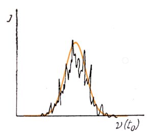
See next illustration – every electron jump after excitation from a higher level (shell) to a lower level (shell) in unique way, (the influence of omnipresent pure chaotic environment like quantum field) See below line spectrum with probability distribution of emitted radiation with two peaks.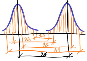
No two wavelenghts are alike. No two wavelenghts has same size. But they have a common denominator – Planck’s constant. Roughly written – Planck’s constant is the peak around which the wavelengths of emitted line spectrum radiation are piled. Planck’s constant slightly changes depending on the “pile-up” of emitted photons
See wavalenghts from upper image 1 > 2 > 3 > 4. The average wavelenght does not really exist. Such wavelenght is only calculated peak of probabilitisc distribution of emitted photons with different wavelenghts. I suppose there are no two wavelengths that are the same in any limited interval. See in mathematics – there can be infinitely many other real numbers in any small limited interval of rational numbers on the number line. These rational numbers differ from each other in ever smaller values.
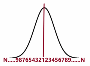
Every wavelenght is unrepeteable original. We can certainly approximate the wavelengths of the emitted radiation in number to a certain number of decimal places. And for calculations with any accuracy, this is necessary. But let’s keep in mind that each wavelength is a non-repeatable, irrational number. Distinguishability of electrons in accordance of their position. Every electron has unique position to each other. Such position could be expressed by irrational number. Very important notice – the course of the real spectrum is very different from the course of the idealized spectrum – See below the difference between orange curve and black course
Let’s go on. Not only each emitted electron is a unique, unrepeatable original, but also each part of the vacuum fluctuation of the quantum field. Particles in form of shaped waves are product of quantum field. They are still influnced by self-similar excitations and excitations of other particlecs (packs of waves).
Very simply written – the quantum field full of random and “shape” non-repeatable vacuum fluctuations is very productive environment for dissipation. It is impossible to exactly repeat any process and even to return to the original conditions before the start of the process. There will always be an unrepeatable change, there will always be a different state from the previous one. The slightest changes at the quantum level in the dimensions of Planck’s constant are very small, but not so small with respect to particles. Especially when we know that particles (the probabilistic appearance of a wave “packet”) are a product (excitations) of this quantum field. These particles therefore respect the environment in which they arise. And the environment – the quantum field – is random and indescribable in all directions. This brings us to the so-called the arrow of time, which is also valid at the micro-level of the quantum field. And not only at the macro level – bodies in mechanics, molecules in thermodynamics.
Example: in mathematics, cryptography, we have one 100% efficient cypher and that is a cypher using a series of random numbers. The principle is that we add the message code in numbers to a series of random numbers. The series of numbers thus added will again be random. The disadvantage of this cypher is double, firstly the series of random numbers must not be repeated and secondly the receiver and sender must first exchange the series of random numbers in some other way. This is the principle – randomness absorbs regularity. And so it is with the quantum field. That’s why particles are constantly being renewed.
Go back to sharp-line spectrum. There are two sharp peaks of radiation with different wavelenghts f1 and f2. See below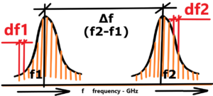
As we see from upper image every wavelenght in sharp probabilistic curve is unrepeteable originall. df1 slightly differs to each other. But there is a common mark – the difference between two peaks ∆f = f2-f1 is much more greater then greater difference df1 or df2.
The same is valid for the appearances of apples and pears in the world. No two apples are exactly alike. It is the same with apples and with all biological species, and indeed with all shapes in the universe – each atom is slightly different from one another, just as one vacuum fluctuation is inexpressibly different from another. See below – “quantized” differences between apples and pears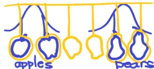
Apples and pears are easily recognizable from each other. This is also valid for the most untypical apples or pears.
Conclusion:
Upper text explains the arrow of time based on the fact purely random behaviour of quantum field. Such quantum field fills the entire universe with all its visible and invisible matter. The indescribable random behaviour means a one directional arrow of time thus also in the case of the collapse of the universe back to the singularity there will be no reversal, but new previously unrepeatable events.
The bound chaos is the source of the arrow of time. Unrepeatable originality in every moment, in every progression, in every change. The whole of Nature is modulated by these purely random chaotic fluctuations. Structures (basic laws, basic appearances) are given – basic features of e.g. species – an apple or a pear or a snowflake. Every snowflake is an unrepeatable original, just as every apple or pear or any other biological species or any chemical substance or chemical element is an unrepeatable original under a strictly given structure – see the hexagonal structure of every different snowflake. No structure is able to support, to sustained itself. No mention how complicated such structures could be. Finally, even chaos itself is unable to support itself in chaos, for chaos cannot sustain itself in chaotic behaviour.
How to measure randomnes or how to find out some order, same meaningfull expressions in series of numbers? See below
……. 01100110010000001110001100101100111111111100000000100000001111000101 ……
Is it a random series or otherwise? When we have to decide if a series of numbers is random or if there is a pattern or order in it – How to do that? And how many numbers are needed in the series for such decision? Are we evaluating the whole series or what if there is a part in the right half of the series. And who’s going to evaluate? Machine or human? Which is a big difference – see colour perception.
If we have a sequence of random numbers with three digits – units, tens, hundreds. E.g. 807, 142, 692, 475, 310, 950, 126, 211, 866. To add ordered numbers to previous serie we also obtain a randomly ordered sequence. But only for units, tens and hundreds. If we add higher or lower orders, we get a structure with clearly predictable thousands and unpredictable hundreds, tens, and ones. The same applies in reverse for tenths, hundredths, and so on.
What is the difference between order and chaos? Order is describable as opposed to chaos. See mathematical functions (sin x, log x, etc.) – a definite order, not allowing for even the slightest exception. Whereas chaos is indescribable. Although in terms of thermodynamics, we can generally describe the behavior of many chaotically moving particles. And here we are in statistical physics. But let’s go back to probability. In terms of frequency distribution, it doesn’t matter if the source (e.g., a coin toss) is regular or purely random – we get the same probability distribution curve for the frequency of tosses.
There is another common denominator between order and chaos. These describable (e.g. log x, x2 ) mathematical functions are very tightly defined without any exception. Very hard prescribe, very reckless to surrounded circumstances. The same situation as with total chaos. Very reckles of the circumstances, also. How to define very beautiful curves like woman´s face? How to define development of shapes from the germ cell through childhood to adulthood? Especially to the final curves of the beautiful female face. A pessimist will say beautiful, but unfortunately only for a limited time. An optimist will say, at least beautiful for a while. And the realist will wonder why that is. Why beauty is so limited in the world, it’s good that it is, but why so briefly.
And a very frequent question – where did such beautiful shapes come from in nature that are neither chaotic nor strictly mathematical?
Or another question. Can there be a probability calculus without distinguishable structures? Whether shape or positionally distinguishable. Imagine an ideal ball, instead of a dice. For every roll of the dice, one of the six sides will land. But what about the ball? Where does it land, at what point? A different one each time! How many rolls of the ideal ball, so many different points. If we throw a 20-sided “ball” (icosahedron) we get one side out of 20. If we throw an N-polyhedron, then the result of the throw will be 1 side out of N.
In conclusion: if we want probability as we know it from ordinary calculations, then we need certain distinguishable bounds, limits. Limits of the number of sides, or positions, lengths, time, shapes or structures. Without distinguishable limits and bounds there can be no probability calculus. The probability depends on the distinguishability of limited structures.
Go back to probability. To better illustrate, let’s have a coin that we toss as many times as we want. Surely, every coin toss is a unique process. But in the end, every coin falls on one side or the other. Heads or tails. Heads will be marked with an I and tails will be marked with a 0. The question is how to predict which side will toss. We cannot answer which side will fall on the next toss – prediction is impossible. We only know, as a frame of reference, that the more tosses, the more the frequencies of occurrence of I and 0 will be equal. The probability of one side falling is still 1/2 – even if the same side falls in succession without interruption. Even if the same side I falls 10 times in a row, it doesn’t mean that the probability for the next toss changes. This moves us into the area of fairness of conditions – a fair coin and a fair toss. If we kept getting one side of the coin in the first 10 tosses, does that mean that the coin or the toss conditions are not fair?
Interesting question – how do we know if a coin is fair? It’s easy to tell, the frequency of I (Heads) will be more or less equal to the frequency of 0 (Tails).
Pure probability is only an ideal state. As ideal as a ideal line or a ideal point. There is no such thing in real nature. It is a human abstraction. We cannot realize an ideal point in the world, in the real natural world, just like an ideal line or an ideal probability.
The Galton board represents to us a probability distribution – see below
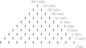
Let’s have a thought experiment. At the beginning of the board with one sharp edge we will have balls falling, regularly alternating left and right. We’ll know exactly where each ball will fall, whether to the left or to the right. If we have 32 balls, they will be regularly divided into 16 balls left and 16 balls right. And the situation is repeated on the two sharp edges in the second row of the Galton board. Again the balls will be regularly divided into two halves on both edges. And this situation will repeat as many times as we have rows of sharp edges.
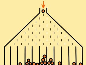
Now let’s have a real experiment with the Galton board. From above we have balls falling, at first on the first row with one sharp edge, and after the division the balls continue to fall on the second row with two edges, then on the third row with three edges, then on the fourth row with four edges, … until …to the Nth row with N sharp edges.
What is the point of the above two experiments? Thought and real? To realize that one ball will keep falling to the right and the other ball will keep falling to the left. This is the case when the initial number of balls is equal to 2N
How is it possible that the balls on one edge do not fall alternately to the right and to the left? In short, why do they fall unpredictably? Once to the right, then to the left and then twice to the right, then again to the left and then five times to the right and then twice to the left then again to the right and then three times to the left?
Why can’t we predict which way the next ball will fall? Only to know the probability of one side is still equal to 1/2 regardless of the falls that have already taken place. Even if any previous series of sides fall, the probability will still be 1/2. Even if the same side falls ten times, the probability will not decrease, but will still be 1/2. How is it possible for a series of 100 identical sides to fall, for example, to the right? That is no longer possible! Yes, it is! It is possible for 1,000,000 equal sides or trillions of trillions of equal sides to fall in unbroken series. Remember the thought experiment, if we have 10 rows on a Galton board, with 210
So the probability depends on the initial number of balls and the number of rows?
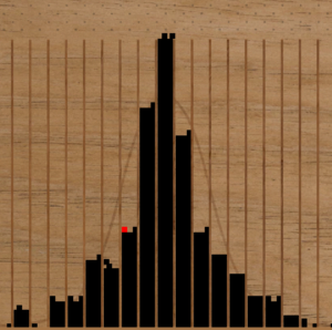
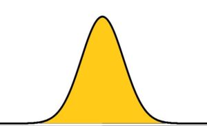
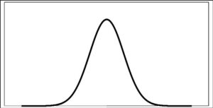
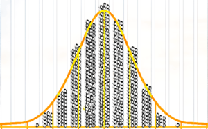
Let us return to realizable experiments. For example, we have a Galton board with 10 rows of sharp edges. The passing of the balls is random, but as a result we get a typical Gaussian curve of the normal distribution of balls after passing through all the rows. See below.
We also know that sometimes, we don’t know when, one ball will keep falling to the right (we can video it and see that was e.g. the 81 ball that kept falling to the right). The question is this – is it possible for the ball that keeps falling to the right to fall at the beginning, in short, to be the first serie? Calculate the probability of this event yourself – you know the number of balls and the number of rows.
And next question – what if the experiment is cancelled? That means, the sharp points of the 10 rows of Galton’s board are not fair, and neither are fair the balls? How do we evaluate the fairness of the conditions?
Galton’s board with 10 rows. Is it possible to have a situation where all the right sides fall at the beginning? Or for the bottom boxes of the board to fill up regularly from right to left according to a Gaussian curve of normal distribution? It is possible, but the probability would be very very low. Just do the analysis for a plate with three rows. Not to mention for 10 or more rows.
A crucial consideration in conclusion on the probability.
We can’t predict what will happen in the microstate (which ball will keep falling to the right), but we can predict the macrostate for a given number of balls versus the number of rows of Galton’s board, that one ball out of 1,024 balls at 10 rows board will keep falling to the right. The nature of probability is the “violation” of regular oscillations (back and forth). In other words, how is it possible for more than one ball to fall on the same side again and again in series of 2, 3, 4, … or N, or N+1 balls?
To be continued next time.
Notice to the Galton board: it’s good to remember that the very first edge, the top edge in the first row, has a probabilistic progression. In other words – already on the first edge the balls will be distributed in an indescribable way. Yes, irregularly and not in alternation, or max two per side and then change sides, or exceptionally three per side, etc. Even at the first edge, the falling balls will alternate two sides in an indescribable way – sometimes on alternate, sometimes two per side, sometimes 10 per side …. and it is possible that 100 or more per side. Or the probability is still 50% regardless of the number of balls already passed. So theoretically you can pass a stabillion balls per side and then change, etc. In short, an inexhaustible wealth of indescribable progressions.
Rather than dealing with these unrealistic but understandable things, it is better to know and experience Reality – Mutuality in the arrangement of forms, colours, structures and events, ovšem i na těchto tzv. neplodných věcech, pakliže jsou vedeny v upřímné touze. Však známe z minulosti kolik tzv. na první pohled neplodných idealistických matematických úvah následně pomohlo v řešení reálných problémů.
Here is only one sharp edge from Galton board. Through such edge the balls gradually pass. See below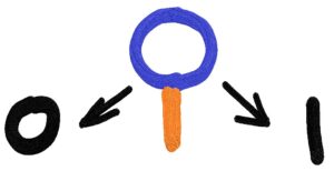
What is the probability of the ball passing through this one edge? What will be the resulting course? We know that the probability P is always 1/2 no matter how many balls have been passed. The balls cannot keep alternating, once to the left (0) and then to the right (I); the balls move unpredictably. So twice in a roll to one side, or three times in a roll to one side, or four times in a roll to one side, or five times in a roll to one side, … , or 10 times in a roll to one side, … , or a hundred times in a roll to one side, … , up to N times in a roll to one side. It is not possible to have a limit that the ball will fall 12 times in a roll to one side and that’s it, because then the probability would not be equal to 1/2. So we will never know what the course of the passing balls will be. However, we do know that the more balls pass, for example 1 million, then one side must land at least twenty times. When 1.26E+30 balls pass, then at least 100 of them must land on the same side. The greater the number of balls passing over the edge the greater the number of balls falling to one side without breaking.
All we care about is the number of passes before the side changes. Certainly, the most common will be a change of sides after one pass – i.e. 0I(I0). And then, with decreasing frequency, changing sides after two, three, … to N passes. See following – I0(1x), II0(2x), III0(3x), IIII0(4x), IIIII0(5x), … , until IIIIIIIII…III(Nx). See below
As we can see from the upper distribution of change frequencies, the most frequent outcome will be a change after 1 pass, i.e. I0 (or 0I), followed by a decrease in frequency for 2 (II0) passes, 3 (III0) passes, and up to N passes.
There is an interesting question: when, during the passage of, say, 1024 balls, will the moment occur when the balls fall 10 times in a series on the same side? Will it happen sometime during the passage, e.g. in the second third or at the beginning?
How to obtain such beautiful course of density function (see below), if we know every event has the same probability?
Yes, every possible event is non-repeteable original. The result is the constant line of density function of realized events. But to obtain very pretty density function (see upper) we have to do something. To ask ourselves for common charasterictis of passing balls or tossed coins – e.g. the appearance of two heads.
a) Imagine modified the Galton board with 4 rows with separating edges only. The function of such board is only to separate passing balls. See below.
How many separations are there, so many boxes. There are 1 + 2 + 4 + 8 separations at 4 rows with 15 edges. Summary thera are 16 collection boxes below. The result is the line of probability distribution.
If we imagine the classical Galton board we see there are separation of passing balls and to connecting partly of them again. To connect passing balls for the next division in the lower row.
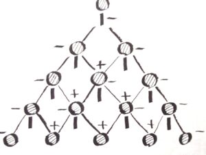
The cancelling of the previous separation and start again with the separation of balls regardless of the previous history of the separation of passed balls. The result? The number of collection boxes is less than the number of collecting boxes in modified Galton board. In other words, there is a slippage between collecting boxes.
In classical Galton board there are 4 rows with 10 edges. In the first row there is only 1 separation of passed balls. In the second row there are 2 separations (-) and 1 reconnecting (+) of passed balls. In the third row there are 3 separations (-) and 2 reconnecting (+) and in the final (fourth) row there are 4 separations (-) and 3 reconnecting (+) of passed balls. When we make a much larger number of rows we ge the resulting “curve” close to the ideal curve of the Gaussian normal probabilistic density function – see below.
Notice: difference between probabilistic distribution and density function is clear from upper image. Probabilistic density function is continuous and smooth, but probabilistic distribution has disconnected appearance – see columns of values.
Now let’s try it quite differently – to the above and mentioned so many times probability distribution or density function. We know that all Nature appears to us always in probability distribution (appearances) of measured parameters. It’s as if everything is hidden in the fog of randomness. But that randomness has quite well-defined areas – see probability appearances all distinguishable shapes, forms or events (processes). The well-known we can also get the Gaussian normal distribution curve in another way. See below

See the upper rope on the support. As can be seen, here probability has no meaning, nor randomness, but only necessity. The shape of the rope is very close to a Gaussian function. See below extracted red rope from the backround of upper image.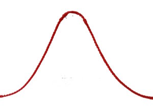
It would be quite difficult to describe mathematically upper “rope course” by using the mechanical properties of the rope. However, this shape can change just as the shape of the Gaussian function changes. Depending on the stiffness of the rope, the elevation of the support, etc. See below – different courses with different supported ropes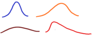
The blue rope has the same stiffness along its entire length. The orange rope has a higher stiffness on its left side. The brown rope has a greater stiffness than the blue rope along its entire length. Whereas the red rope has a high stiffness on its right side and a low stiffness on its left side. Thus, by using different ropes with different stiffnesses, we can get all possible combinations of probability frequency distributions – density functions.
We have two methods to achieve a normal distribution. First method is the passing through the Galton board, second method is the supported rope. These two methods has a common denominator – the maximum around which cumulate all states with a value lower than the maximum value. How to verify fair conditions of every row in the board? See below.
To find the fairness of the conditions, i.e. that each tip (edge) in each row gives a 50%/50% distribution, then we need to pass min. 2N balls, where N is the number of rows in the board (see above for details). Then we obtain upper orange illustrated probability density function which smoothly shows probabilistic distribution of balls in lower boxes. What about probability? Instead probability there is a necessity or certainty. We have certainty, even 100% certainty how the distribution of balls in the lower boxes will look like. Even if we run thousands or trillions of trials, the distribution of balls will still be the same, see the top orange curve. So we get 100% certainty of the result. What about randomness? That’s submitted to the whole. A whole composed of many purely random events. A microstate subordinate to a macrostate. The course of filling the lower boxes will always be different and unpredictable, thus purely random. But the result will always be “the same”. “Same” is in quotes because even the progression of the resulting smoothed (orange) function will be slightly different each time.
As with snowflakes, no two snowflakes are perfectly identical. And what they’ve fallen on the earth over the ages. So are the appearances of biological species or minerals and, indeed, chemical elements. There are no two absolutely identical atoms of hydrogen and of course of all the more massive elements in the world. First of all, I mean the distribution of orbitals of the probable appearance of electrons. Not to mention the influence of the surrounding matter (quantum) field.
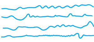
There is a next peculiarity – to have infinity (Galton) board, resp. with very wide limits. What does it mean? It means the following See below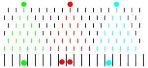
There are only three kind of balls (green, red and blue) and thus three Galton “boards”. But we can combine more balls and more modes of their passage through the board. We have infinity possibilities to different courses in lower boxes. The resulting courses in the lower boxes can have the form of regular oscillations or different shapes up to a purely random distribution of balls. See below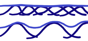
… to be continued – Primordial forms of fair conditions.
There is a parable – probability, certainty and necessity. See the difference between rational and irrational numbers. A rational number is clear, it has a given number of decimal places, any sequence of numbers that repeats to infinity. Irrational numbers also have a sequence of numbers up to infinity. Only we don’t know the sequence, we have to determine it, to calculate it. Maybe to trillions of trillions of decimal numbers. But we never know what the sequence of numbers will be. We don’t know until we calculate it, determine it, in short, until the process of determination, takes place. And it is the same in the passage of balls through the Galton board – we don’t know what the sequence will be until we make the process.
See below a table. There are topics (considerations and suggestions) on the subject of this section. If you want, download the pdf file.
| Download | Download | Download | Download |
| Probability_meaning | Ideal_versus_Real_Probability | ||
| The_probability_1 | |||
| The_probability_2 | |||